6.2 Setting up the magic angle gradient

Before the magic angle gradient can be used in a routine fashion a few adjustments have to be made. In order to ensure short rise and fall times of the pulsed field gradients it is necessary to compensate for Eddy currents generated by the gradient pulses and for the switching times of the gradient amplifier. This is done through so-called pre-emphasis adjustment. Furthermore the gradient strength needs to be calibrated. Before initiating these adjustment procedures make sure that the gradient amplifier has been installed correctly.

 

Adjusting the pre-emphasis

 

Figure 6.3. Pre-emphasis controller window.

 

For this procedure use a rotor with H 2 O/D 2 O, preferably doped with CuSO 4 (2 mMol). Spin the sample at approximately 3 kHz, lock and shim to a proton line width of better than 5 Hz at half height.

 

Set the offset a few kHz off resonance from the water peak. Use a sweep width of 20 ppm, D1=1-2s, and choose TD such that the FID has decayed about 50% in amplitude after approximately 1/8 th of the acquisition time.

 

Next set the pulse program to preempgs (for RX22 based systems set the second channel to proton as well). Use a gradient program which defines a single square gradient pulse (e.g. gradprog=1 squa) and define a variable delay list (vdlist= pre-emp) which contains the following values:
 

100 l, 300 l, 1m, 3m, 10m, 30m, 100m, 300m.

This pulse program will acquire 8 FID's and display them sequentially in a single acquisition window (see figure 6.4). Each FID is acquired at a time vd after a gradient pulse. Set the gradient pulse length to 50 ms and its strength to 20%.

The pre-emphasis is controlled by a set of three time constants and amplitudes. These values can be addressed through the Pre-emphasis Controller window, which is invoked by setpre (figure 6.3). Select for the time constants 20 ms, 2 ms and 200 s and start with 50% for all time settings and 0% for all gain settings.

 

Start the acquisition in gs mode and observe the FID's in the acquisition window. With the time constants set as described above, the first FID's will seem distorted, as can be seen in the example of figure 6.4 (top spectra). Adjust the pre-emphasis values by changing the time constants and gain settings. Start with the settings for the slowest time constant and adjust the 5 th and 6 th FID, so that they appear similar to the last two FID's. Repeat the procedure for the mid and fast time constants, for FID's 3 and 4, and FID's 1 and 2, respectively. If all values are set correctly all FID's should appear equal (figure 6.4, bottom).

 

The pre-emphasis values are dependent on both the probe and the gradient amplifier and once correctly set up, will remain the same. The settings can be stored on the computer by saving the set-up from the file menu in the Pre-emphasis Controller window.

 

Figure 6.4. 8 consecutive FID's Acquired at different times after the application of a gradient pulse. Top: without

pre-emphasis; bottom: with pre-emphasis properly adjusted.

 

Calibrating the gradient

 

Gradient calibration is performed by measuring the gradient profile of a sample of known size. Usually a proton spectrum of a sample of water is acquired.

The profile is obtained with a gradient spin-echo, which can be acquired with the pulse program calib. Set the gradient amplifiers to a low output, e.g. 10 or 20% and acquire 4 scans. Multiply the FID with a sinebell (ssb=0), Fourier transform and represent the data in magnitude mode (mc). The resulting profile represents a projection of the sample's density along the magic angle spinner axis. For a sample of known length the gradient strength can be determined by measuring the width of the spectrum ( ) and dividing it by the length of the sample (l, in cm), by the gyromagnetic constant of protons ( =4250 Hz/G) and by the current of the gradient amplifier (I in A):

 

 

 

 

In figure 6.5 below, water in a spherical insert is used to calibrate the gradient strength. The profile represents the spherical sample volume plus a small amount of water in the fill hole of the inserts. From the width of the profile ( =12000 Hz) and the known length of the sample (l=0.27 cm) and gradient amplifier output (20% of 10A), the gradient strength is determined as 5.2 Gcm -1 A -1 .

 

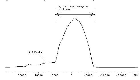
Figure 6.5. Gradient profile for a spherical sample of water. The gradient strength is obtained from the width of the profile.